
Overview
The Excel REDUCE function reduces an array to an accumulated value by applying a LAMBDA function to each value and returning the total value in the accumulator.
Syntax
=REDUCE(initial_value, array, function)
Arguments
initial_value – The starting value for the accumulator.
array – The array to be reduced.
function – A LAMBDA that is called to reduce the array.
Version
Excel 365
Purpose
The Excel REDUCE function applies a custom LAMBDA function to each value in the input array and returns an accumulated value.
=OR(logical1, [logical2], …)
Examples
Let’s take a look at how we can use the OR function in it’s simplest form:
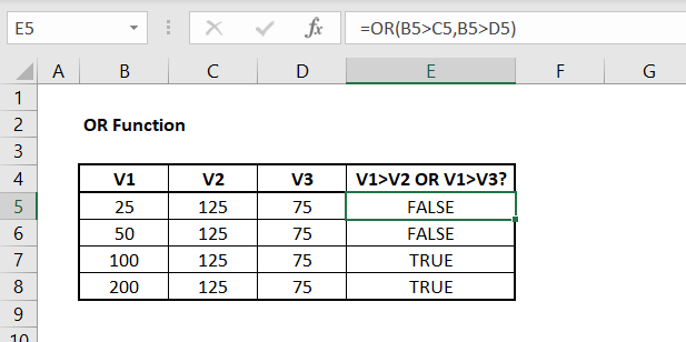
The formula we have in cell E5 (and is applied to the adjacent cells in column E) is:
=OR(B5 > C5, B5 > D5)
In column E, we are looking to understand if V1 is greater than either V2 or V3. For row 5, we see that V1 is 25, which is less than V2 at 125 and less than V3 at 75. As such, the OR function evaluates to FALSE since V1 is not greater than V2 or V3.
However, when we get down to row 7, we see that V1 is now greater than V3. Although it is still less than V2, only one conditions needs to evaluate as TRUE in the OR function for the OR function to return TRUE.
The OR function will always return either TRUE or FALSE, which may not be effective in communicating what you want from the function. Instead, we can pair the OR function with the IF function:
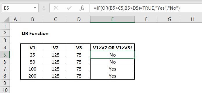
The formula we have in cell E5 (and is applied to the adjacent cells in column E) is:
Here we have combined the IF function with the OR function to change the output of the result. Instead of the OR function returning TRUE or FALSE, now we see either “Yes” or “No” as the output.
There also may be the case where you want to see the inverse result of the OR function. In this example, we are using the NOT function to ensure the OR function returns FALSE if any individual argument evaluates as TRUE:
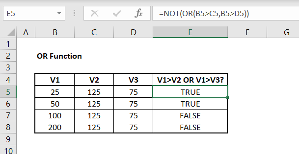
The formula we have in cell E5 (and is applied to the adjacent cells in column E) is:
Here we can see the output of the OR function is opposite to what we saw in the first example, above. Since the OR function only returns TRUE if any single argument is TRUE, combining the OR function and NOT function can be useful in situations where you want the opposite result.
Notes
- The logical condition(s) must evaluates as either TRUE or FALSE or a #VALUE error will occur
- Text values or empty cells entered as arguments will be ignored
Author

Kyle Stott
Certified Microsoft Excel Expert
Kyle has worked professionally with Microsoft Excel for over a decade and has been consulting on and teaching best practices in Microsoft Excel to over 400 companies across 30+ countries.
Want to learn more?
Join My Excel Academy Today!
This All-Access Pass Includes:

- Access to All My Excel Academy Courses
- 20+ hours of on-demand video
- 1-on-1 instructor support
- Mobile learning supported
- Frequently updated content
- Learn at your own pace
- 500+ practice problems
- Certificate of completion
30-Day Money-Back Guarantee
Want to learn more?
Join My Excel Academy Today!
All-Access Pass Includes:
- Access to All My Excel Academy Courses
- 20+ hours of on-demand video
- 1-on-1 instructor support
- Mobile learning supported
- Frequently updated content
- Learn at your own pace
- 500+ practice problems
- Certificate of completion
30-Day Money-Back Guarantee
Want to learn more?
Join My Excel Academy Today!
30-Day Money-Back Guarantee
This all-access pass includes:
- Access to all My Excel Academy Courses
- 20+ hours of on-demand video
- 1-on-1 instructor support
- Mobile learning supported
- Frequently updated content
- Learn at your own pace
- 500+ practice problems
- Certificate of completion
Don’t hesitate – join now!