Overview
The Excel IFS function checks whether one or more conditions are met and returns the corresponding value to the first TRUE condition. The IFS function essentially replaces the need for multiple nested IF statements and as such, is much easier to read.
Syntax
=IFS(logical_test1, value_if_true1, [logical_test2], [value_if_true2], …)
Arguments
logical_test1 – Any value or expression that can be evaluated to TRUE or FALSE.
value_if_true1 – The value returned if logical_test1 is TRUE.
logical_test2 – [optional] Second value or expression that can be evaluated to TRUE or FALSE.
value_if_true2 – [optional] The value returned if logical_test2 is TRUE.
Version
Excel 2019 and onward
Purpose
The IFS function evaluates one or more logical tests and returns the corresponding value for the first TRUE condition. The IFS function was introduced in Excel to remove the need for nesting IF statements, which can be difficult to read.
The IFS function allows you to test up to 127 different conditions. In other words, the IFS function will work through each logical test sequentially, until one of the logical tests evaluates as TRUE. Once a logical test evaluates as TRUE, the corresponding result value will be returned. In the event multiple conditions in the formula evaluate as TRUE, only the first TRUE result will be returned. As such, it’s important to consider the order of the logical tests in the IFS function. The IFS function will process and evaluate logical tests from first-to-last (left-to-right), as written.
=IFS(
logical_test1, value_if_true1 // evaluated 1st
logical_test2, value_if_true2 // evaluated 2nd
)
Examples
Let’s look at a few examples of how we can use the IFS function.
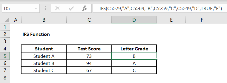
In this first example, we’ll assign a letter grade to a corresponding test score. Using the following data set, we get:

The formula we have in cell D5 (and apply to the cells below) is:
=IFS(C5>79, “A”, C5>69, “B”, C5>59, “C”, C5>49, “D”, TRUE, “F”)
Here we see that cell D5 evaluates to “B”, since the first logical test that is TRUE in the above formula is ‘C5>69’. Reading left-to-right, C5 is not greater than 79, so the first argument evaluates as FALSE. However, C5 is greater than 69, so the formula returns “B”. Although cell C5 is also greater than 59 and 49, the IFS function returns the first TRUE value.
Lastly, you’ll see our final logical test has the value ‘TRUE’. In this case, we know if the student scores 49 or less, they have failed, or scored an ‘F’. As such, we want the last logical test to evaluate as TRUE regardless, so we can just use TRUE as a catch-all default to ensure this happens (if all other logical tests evaluate to FALSE).
To demonstrate the value of the IFS function, below is the syntax for a nested IF function, which accomplishes the same functionality as the IFS formula we created above:
Instead of using one IFS function, here we needed to use four nested IF statements to achieve the same result, which can be very tedious to read and troubleshoot for errors as the number of conditions increase.
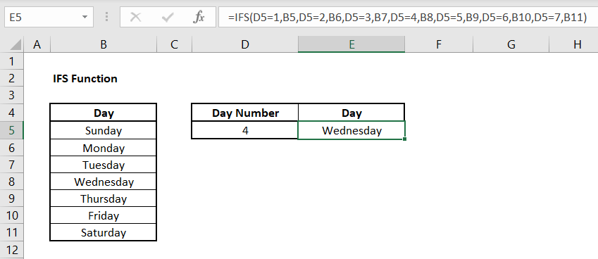
In this next example, let’s determine which day of the week it is, based on a numerical number:

The formula we have in cell E5 is:
=IFS(D5=1, B5, D5=2, B6, D5=3, B7, D5=4, B8, D5=5, B9, D5=6, B10, D5=7, B11)
This setup assumes Sunday = 1, Monday = 2, Tuesday = 3, etc.
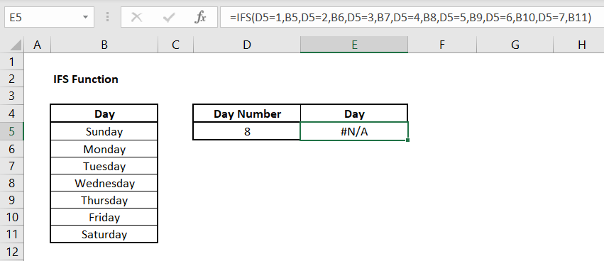
Now, let’s assume the user enters a values that’s not accepted, like 8. We would get:

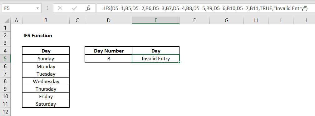
Here we see an #N/A error appear, as the corresponding result for 8 is ‘Not Available’. Although there are many ways to handle #N/A errors, such as the IFNA function or IFERROR function, we can also handle the error directly in the IFS function with a final catch-all condition, seen below:

The final catch-all condition, which automatically evaluates as TRUE, will inform the user that their entry is invalid. The formula can be seen below:
=IFS(D5=1, B5, D5=2, B6, D5=3, B7, D5=4, B8, D5=5, B9, D5=6, B10, D5=7, B11, TRUE, “Invalid Entry”)
Notes
- The IFS function can support up to 127 different conditions
- The IFS function does not have a default value if all conditions are FALSE – this will result in a #N/A error
- To include a default value if all conditions are FALSE, use TRUE as your final logical test
- If any logical tests do not evaluate to either TRUE or FALSE, this will result in a #VALUE! error
Author

Kyle Stott
Certified Microsoft Excel Expert
Kyle has worked professionally with Microsoft Excel for over a decade and has been consulting on and teaching best practices in Microsoft Excel to over 400 companies across 30+ countries.
Want to learn more?
Join My Excel Academy Today!
This All-Access Pass Includes:

- Access to All My Excel Academy Courses
- 20+ hours of on-demand video
- 1-on-1 instructor support
- Mobile learning supported
- Frequently updated content
- Learn at your own pace
- 500+ practice problems
- Certificate of completion
30-Day Money-Back Guarantee
Want to learn more?
Join My Excel Academy Today!

All-Access Pass Includes:
- Access to All My Excel Academy Courses
- 20+ hours of on-demand video
- 1-on-1 instructor support
- Mobile learning supported
- Frequently updated content
- Learn at your own pace
- 500+ practice problems
- Certificate of completion
30-Day Money-Back Guarantee

Want to learn more?
Join My Excel Academy Today!
30-Day Money-Back Guarantee
This all-access pass includes:
- Access to all My Excel Academy Courses
- 20+ hours of on-demand video
- 1-on-1 instructor support
- Mobile learning supported
- Frequently updated content
- Learn at your own pace
- 500+ practice problems
- Certificate of completion
Don’t hesitate – join now!
