Overview
The Excel MAP function returns an array formed by mapping each value in the array to a new value by applying a LAMBDA to create a new value. A LAMBDA is applied to each value in the mapped array and the result is a new array of the same size, with results from the LAMBDA.
Syntax
=MAP(array1, [array2, …], lambda)
Arguments
array1 – The first array to be mapped.
array2 – [optional] The second array to be mapped.
lambda – A LAMBDA to be applied to each value in the mapped array(s).
Version
Excel 365
Purpose
The Excel MAP function returns an array formed by mapping each value in the array to a new value by applying a LAMBDA to create a new value. A LAMBDA is applied to each value in the mapped array and the result is a new array of the same size, with results from the LAMBDA.
The MAP function is valuable for when you want to apply a calculation to several fields within a range or array and want to output the results as an array. The MAP function has two required arguments: array1 and lambda. Array1 is the array to be mapped. Lambda is the LAMBDA function that performs a calculation on each item within the mapped array. Additional arrays can be included in the MAP function before lambda, if desired.
=MAP(array1, [array2], lambda)
Examples
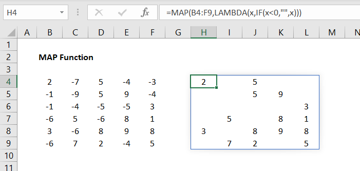
In this first example, we’ll check each value in the target array and see which are less than 0. If a value is less than zero, we’ll have the word “ERROR” appear in the output array and if a value is greater than zero, we’ll have whatever number it is in the input array appear in the output array.

The formula we have in cell H4 (and spills to adjacent cells) is:
In the example above, the range ‘B4:F9’ is our array1 value. We then apply a LAMBDA to that range that uses an IF function to determine if values within the range are less than 0. One of the benefits of the MAP function is that it will automatically spill to the size of your input array. In the example above, we only need to enter the MAP function (with it’s arguments) into cell H4.
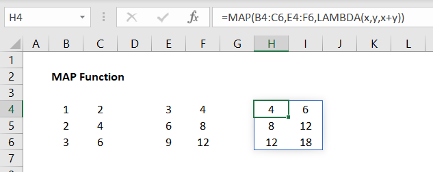
The MAP function can also be used with multiple input arrays. In the example below, we can quickly add two arrays together:

The formula we have in cell H4 is:
Here we have two input arrays: ‘B4:C6’ is array1 and ‘E4:F6’ is array2. We then use a LAMBDA to add ‘x’ and ‘y’ together, where ‘x’ relates to array1 and ‘y’ relates to array2.
It’s not always necessary or beneficial to use the MAP function as the functionality can be achieved through other means. However, the two main reasons to use the MAP function are:
- To run logical tests with the IF, AND, OR or NOT functions. Since all logical functions result in a single value, it can be beneficial to use the MAP function to quickly map array(s) to a new array.
- To make a function spill that otherwise wouldn’t.
Notes
- An invalid LAMBDA function or an incorrect number of parameters will return a #VALUE! error
- The MAP function returns an array of results. If you want a single aggregate result, the REDUCE function can be used
Author

Kyle Stott
Certified Microsoft Excel Expert
Kyle has worked professionally with Microsoft Excel for over a decade and has been consulting on and teaching best practices in Microsoft Excel to over 400 companies across 30+ countries.
Want to learn more?
Join My Excel Academy Today!
This All-Access Pass Includes:

- Access to All My Excel Academy Courses
- 20+ hours of on-demand video
- 1-on-1 instructor support
- Mobile learning supported
- Frequently updated content
- Learn at your own pace
- 500+ practice problems
- Certificate of completion
30-Day Money-Back Guarantee
Want to learn more?
Join My Excel Academy Today!

All-Access Pass Includes:
- Access to All My Excel Academy Courses
- 20+ hours of on-demand video
- 1-on-1 instructor support
- Mobile learning supported
- Frequently updated content
- Learn at your own pace
- 500+ practice problems
- Certificate of completion
30-Day Money-Back Guarantee

Want to learn more?
Join My Excel Academy Today!
30-Day Money-Back Guarantee
This all-access pass includes:
- Access to all My Excel Academy Courses
- 20+ hours of on-demand video
- 1-on-1 instructor support
- Mobile learning supported
- Frequently updated content
- Learn at your own pace
- 500+ practice problems
- Certificate of completion
Don’t hesitate – join now!
